The effect of over-sampling and under-sampling on model calibration#

This note book examines the effect of under-sampling or over-sampling (including SMOTE) to balance training examples for imbalanced data, and shows alternative methods of recalibrating the model.

Note: a well-calibrated model is especially important when model prediction probabilities are read as risks (e.g. risk of emergency hopsital admission for any given patient).

Observations#

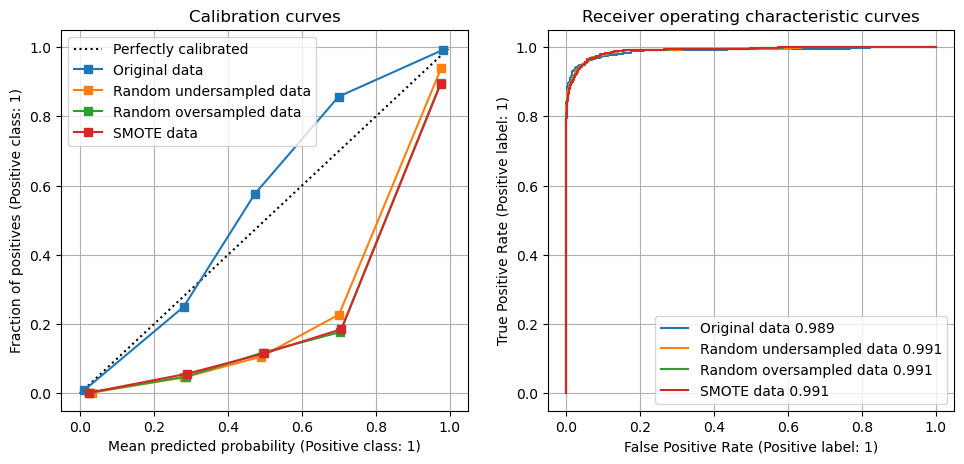
Using under-sampling or over-sampling to balance classes in training and test sets improved the recall of the model, at the expense of the precision of the model. Use of under-sampling or over-sampling led to an overestimation of the frequency of the minority class, and led to significant perturbation of the model calibration.

Recalibration of the model could restore calibration accuracy (at the loss of improved recall). The best calibration type was beta-calibration (https://pypi.org/project/betacal/).

Load packages#

# Install beta calibration package if not installed

try:
    import betacal
except:
    !pip install betacal

import matplotlib.pyplot as plt
import numpy as np

from imblearn.over_sampling import SMOTE
from imblearn.over_sampling import RandomOverSampler
from imblearn.under_sampling import RandomUnderSampler

from betacal import BetaCalibration

from sklearn.calibration import CalibrationDisplay
from sklearn.datasets import make_classification
from sklearn.isotonic import IsotonicRegression
from sklearn.linear_model import LogisticRegression
from sklearn.linear_model import LogisticRegression
from sklearn import metrics

from sklearn.model_selection import train_test_split

Generate data set#

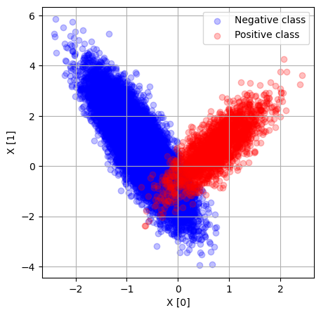
We will generate a set of data where 90% of examples are the negative class, and 10% the positive class.

X, y = make_classification(n_samples=20000, n_features=2, n_redundant=0,
        n_clusters_per_class=1, weights=[0.90, 0.10], class_sep=0.75, flip_y=0,
        hypercube=True, random_state=42)

fig = plt.figure(figsize=(5,5))
ax = fig.add_subplot() 
mask = y == 0
ax.scatter (X[mask, 0], X[mask, 1], c='b', alpha=0.25, label='Negative class')
mask = y == 1
ax.scatter (X[mask, 0], X[mask, 1], c='r', alpha=0.25, label='Positive class')
ax.legend()
ax.set_xlabel('X [0]')
ax.set_ylabel('X [1]')
ax.grid()
plt.show()

_images/51_sampling_and_calibration_6_0.png

Split into training, test and calibration check sets#

# Split full data into training and test sets
X_train, X_test, y_train, y_test = train_test_split(
    X, y, test_size=0.5, random_state=42, stratify=y)

# Split test into test and calibration check 
X_cal, X_test, y_cal, y_test = train_test_split(
    X_test, y_test, test_size=0.5, random_state=42, stratify=y_test)

# Expand training set with SMOTE
smote = SMOTE(random_state=42)
X_smote, y_smote = smote.fit_resample(X_train, y_train)

Fit model to original data and oversampled or undersampled data#

Note what happens to ROC AUC, recall (what proportion of actual positives was identified correctly?), precision (what proportion of positive identifications was actually correct?), and predicted positive rate (the real data has a positive rate of 0.10).

Fit model to original data balance#

model = LogisticRegression()
model.fit(X_train, y_train)

# Get acuracy scores
auc = metrics.roc_auc_score(y_test, model.predict_proba(X_test)[:,1])
print (f'ROC AUC: {auc:0.3f}')

recall = metrics.recall_score(y_test, model.predict(X_test))
print (f'Recall: {recall:0.3f}')

precision = metrics.precision_score(y_test, model.predict(X_test))
print (f'Precision: {precision:0.3f}')

predicted_positive_rate = model.predict_proba(X_test)[:,1].mean()
print (f'Predicted positive rate: {predicted_positive_rate:0.3f}')

ROC AUC: 0.989
Recall: 0.866
Precision: 0.982
Predicted positive rate: 0.100

Fit model to randomly oversampled majority data#

oversampler = RandomOverSampler(random_state=42)
X_oversampled, y_oversampled = oversampler.fit_resample(X_train, y_train)

model_oversampled = LogisticRegression()
model_oversampled.fit(X_oversampled,y_oversampled)

# Get acuracy scores
auc = metrics.roc_auc_score(y_test, model_oversampled.predict_proba(X_test)[:,1])
print (f'ROC AUC: {auc:0.3f}')

recall = metrics.recall_score(y_test, model_oversampled.predict(X_test))
print (f'Recall: {recall:0.3f}')

precision = metrics.precision_score(y_test, model_oversampled.predict(X_test))
print (f'Precision: {precision:0.3f}')

predicted_positive_rate = model_oversampled.predict_proba(X_test)[:,1].mean()
print (f'Predicted positive rate: {predicted_positive_rate:0.3f}')

ROC AUC: 0.991
Recall: 0.942
Precision: 0.725
Predicted positive rate: 0.158

Fit model to SMOTE over-sampled data#

smote = SMOTE(random_state=42)
X_smote, y_smote = smote.fit_resample(X_train, y_train)

model_smote = LogisticRegression()
model_smote.fit(X_smote, y_smote)

# Get acuracy scores
auc = metrics.roc_auc_score(y_test, model_smote.predict_proba(X_test)[:,1])
print (f'ROC AUC: {auc:0.3f}')

recall = metrics.recall_score(y_test, model_smote.predict(X_test))
print (f'Recall: {recall:0.3f}')

precision = metrics.precision_score(y_test, model_smote.predict(X_test))
print (f'Precision: {precision:0.3f}')

predicted_positive_rate = model_smote.predict_proba(X_test)[:,1].mean()
print (f'Predicted positive rate: {predicted_positive_rate:0.3f}')

ROC AUC: 0.991
Recall: 0.942
Precision: 0.722
Predicted positive rate: 0.158

Fit model to random undersampled majority data#

undersampler = RandomUnderSampler(random_state=42)
X_undersampled, y_undersampled = undersampler.fit_resample(X_train, y_train)

model_undersampled = LogisticRegression()
model_undersampled.fit(X_undersampled,y_undersampled)

# Get acuracy scores
auc = metrics.roc_auc_score(y_test, model_undersampled.predict_proba(X_test)[:,1])
print (f'ROC AUC: {auc:0.3f}')

recall = metrics.recall_score(y_test, model_undersampled.predict(X_test))
print (f'Recall: {recall:0.3f}')

precision = metrics.precision_score(y_test, model_undersampled.predict(X_test))
print (f'Precision: {precision:0.3f}')

predicted_positive_rate = model_undersampled.predict_proba(X_test)[:,1].mean()
print (f'Predicted positive rate: {predicted_positive_rate:0.3f}')

ROC AUC: 0.991
Recall: 0.942
Precision: 0.745
Predicted positive rate: 0.163

Show calibration curves for models trained on data sets#

fig = plt.figure(figsize=(10,5))

# Calibration
ax1 = fig.add_subplot(121)
disp1 = CalibrationDisplay.from_estimator(
    model, X_test, y_test, ax=ax1, n_bins=5, label='Original data')
disp2 = CalibrationDisplay.from_estimator(
    model_undersampled, X_test, y_test, ax=ax1, n_bins=5, label='Random undersampled data')
disp3 = CalibrationDisplay.from_estimator(
    model_oversampled, X_test, y_test, ax=ax1, n_bins=5, label='Random oversampled data')
disp4 = CalibrationDisplay.from_estimator(
    model_smote, X_test, y_test, ax=ax1, n_bins=5, label='SMOTE data')
ax1.legend(loc='upper left')
ax1.set_title('Calibration curves')
ax1.grid()

# ROC
ax2 = fig.add_subplot(122)

auc = metrics.roc_auc_score(y_test, model.predict_proba(X_test)[:,1])
disp1 = metrics.RocCurveDisplay.from_estimator(
    model, X_test, y_test, ax=ax2, label=f'Original data {auc:0.3f}')

auc = metrics.roc_auc_score(y_test, model_undersampled.predict_proba(X_test)[:,1])
disp2 = metrics.RocCurveDisplay.from_estimator(
    model_undersampled, X_test, y_test, ax=ax2, label=f'Random undersampled data {auc:0.3f}')

auc = metrics.roc_auc_score(y_test, model_oversampled.predict_proba(X_test)[:,1])
disp3 = metrics.RocCurveDisplay.from_estimator(
    model_oversampled, X_test, y_test, ax=ax2, label=f'Random oversampled data {auc:0.3f}')

auc = metrics.roc_auc_score(y_test, model_smote.predict_proba(X_test)[:,1])
disp4 = metrics.RocCurveDisplay.from_estimator(
    model_smote, X_test, y_test, ax=ax2, label=f'SMOTE data {auc:0.3f}')

ax2.set_title('Receiver operating characteristic curves')
ax2.grid()

plt.tight_layout(pad=2)
plt.show()

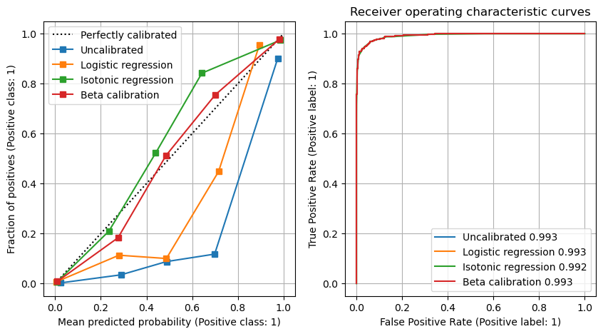
_images/51_sampling_and_calibration_20_0.png

Calibrate model results with three methods#

We will calibrate the data with three methods:

Logistic regression (Platt sclaing)
Isotonic regresssion
Beta calibratio (betacal)

Here will will demonstrate these methods with SMOTE oversampling.

We will fit the calibrator to the test data, and test against the calibration check data.

Model fitted to raw SMOTE data without calibration#

# Get calibration check set predictions
cal_proba = model_smote.predict_proba(X_cal)[:,1]
cal_proba = cal_proba.reshape(-1, 1)

# Get acuracy scores
auc = metrics.roc_auc_score(y_cal, cal_proba)
print (f'ROC AUC: {auc:0.3f}')

recall = metrics.recall_score(y_cal, cal_proba >= 0.5)
print (f'Recall: {recall:0.3f}')

precision = metrics.precision_score(y_cal, cal_proba >= 0.5)
print (f'Precision: {precision:0.3f}')

predicted_positive_rate = np.mean(cal_proba >= 0.5)
print (f'Predicted positive rate: {predicted_positive_rate:0.3f}')

ROC AUC: 0.993
Recall: 0.948
Precision: 0.714
Predicted positive rate: 0.133

SMOTE fit calibrated with logistic regression#

# Get test set predicitons
smote_test_pred = model_smote.predict_proba(X_test)[:,1]
smote_test_pred = smote_test_pred.reshape(-1, 1)

# Fit logistic calibrator
lr = LogisticRegression(C=9999)
lr.fit(smote_test_pred, y_test)

# Get calibrated probablilities
lr_calibrated = lr.predict_proba(cal_proba)

# Get acuracy scores
auc = metrics.roc_auc_score(y_cal, lr_calibrated[:,1])
print (f'ROC AUC: {auc:0.3f}')

recall = metrics.recall_score(y_cal, lr_calibrated[:,1] >= 0.5)
print (f'Recall: {recall:0.3f}')

precision = metrics.precision_score(y_cal, lr_calibrated[:,1] >= 0.5)
print (f'Precision: {precision:0.3f}')

predicted_positive_rate = np.mean(lr_calibrated[:,1] >= 0.5)
print (f'Predicted positive rate: {predicted_positive_rate:0.3f}')

ROC AUC: 0.993
Recall: 0.928
Precision: 0.874
Predicted positive rate: 0.106

SMOTE fit calibrated with isotonic regression#

# Fit isotonic calibrator
iso = IsotonicRegression()
iso.fit(smote_test_pred, y_test)

# Get calibrated probablilities
iso_calibrated = iso.predict(cal_proba)

# Get acuracy scores
auc = metrics.roc_auc_score(y_cal, iso_calibrated)
print (f'ROC AUC: {auc:0.3f}')

recall = metrics.recall_score(y_cal, iso_calibrated >= 0.5)
print (f'Recall: {recall:0.3f}')

precision = metrics.precision_score(y_cal, iso_calibrated >= 0.5)
print (f'Precision: {precision:0.3f}')

predicted_positive_rate = np.mean(iso_calibrated >= 0.5)
print (f'Predicted positive rate: {predicted_positive_rate:0.3f}')

ROC AUC: 0.992
Recall: 0.862
Precision: 0.956
Predicted positive rate: 0.090

SMOTE fit calibrated with beta regression#

# Fit isotonic calibrator
beta = BetaCalibration(parameters="abm")
beta.fit(smote_test_pred, y_test)

# Get calibrated probablilities
beta_calibrated = beta.predict(cal_proba)

# Get acuracy scores
auc = metrics.roc_auc_score(y_cal, beta_calibrated)
print (f'ROC AUC: {auc:0.3f}')

recall = metrics.recall_score(y_cal, beta_calibrated >= 0.5)
print (f'Recall: {recall:0.3f}')

precision = metrics.precision_score(y_cal, beta_calibrated >= 0.5)
print (f'Precision: {precision:0.3f}')

predicted_positive_rate = np.mean(beta_calibrated >= 0.5)
print (f'Predicted positive rate: {predicted_positive_rate:0.3f}')

ROC AUC: 0.993
Recall: 0.882
Precision: 0.946
Predicted positive rate: 0.093

fig = plt.figure(figsize=(10,5))

# Calibration

ax1 = fig.add_subplot(121)

disp1 = CalibrationDisplay.from_predictions(y_cal, cal_proba,
     ax=ax1, n_bins=5, label='Uncalibrated')

disp2 = CalibrationDisplay.from_predictions(y_cal, lr_calibrated[:, 1],
     ax=ax1, n_bins=5, label='Logistic regression')

disp3 = CalibrationDisplay.from_predictions(y_cal, iso_calibrated,
     ax=ax1, n_bins=5, label='Isotonic regression')

disp4 = CalibrationDisplay.from_predictions(y_cal, beta_calibrated,
     ax=ax1, n_bins=5, label='Beta calibration')

ax1.grid()
ax1.legend(loc='upper left')


# ROC
ax2 = fig.add_subplot(122)

auc = metrics.roc_auc_score(y_cal, cal_proba)
disp1 = metrics.RocCurveDisplay.from_predictions(
    y_cal, cal_proba, ax=ax2, label=f'Uncalibrated {auc:0.3f}')

auc = metrics.roc_auc_score(y_cal, lr_calibrated[:,1])
disp2 = metrics.RocCurveDisplay.from_predictions(y_cal, lr_calibrated[:, 1], 
    ax=ax2, label=f'Logistic regression {auc:0.3f}')

auc = metrics.roc_auc_score(y_cal, iso_calibrated)
disp3 = metrics.RocCurveDisplay.from_predictions(y_cal, iso_calibrated,
    ax=ax2, label=f'Isotonic regression {auc:0.3f}')

auc = metrics.roc_auc_score(y_cal, beta_calibrated)
disp4 = metrics.RocCurveDisplay.from_predictions(y_cal, beta_calibrated,
    ax=ax2, label=f'Beta calibration {auc:0.3f}')

ax2.set_title('Receiver operating characteristic curves')
ax2.grid()

plt.show()

_images/51_sampling_and_calibration_31_0.png

Observations#

Recalibration of the model could restore calibration accuracy (at the loss of improved recall). The best calibration type was beta-calibration (https://pypi.org/project/betacal/).

Titanic Survival Machine Learning

The effect of over-sampling and under-sampling on model calibration

Contents

The effect of over-sampling and under-sampling on model calibration#

Observations#

Load packages#

Generate data set#

Split into training, test and calibration check sets#

Fit model to original data and oversampled or undersampled data#

Fit model to original data balance#

Fit model to randomly oversampled majority data#

Fit model to SMOTE over-sampled data#

Fit model to random undersampled majority data#

Show calibration curves for models trained on data sets#

Calibrate model results with three methods#

Model fitted to raw SMOTE data without calibration#

SMOTE fit calibrated with logistic regression#

SMOTE fit calibrated with isotonic regression#

SMOTE fit calibrated with beta regression#

Observations#