A comparison of calibration of neural networks using a single sigmoid output or dual SoftMax or Sigmoid outputs
Contents
A comparison of calibration of neural networks using a single sigmoid output or dual SoftMax or Sigmoid outputs#
When constructing a neural network to distinguish between two classifications (e.g. survived vs died), we have two options with neural networks:
Provide an output for each, with the probability of each being reported, e.g. died=84%, survived=16%. In this case we can use Sigmoid output which treats each class as independent, or SoftMax to ensure that the probabilities add up to 1.0.
Provide an output for just one of the options, e.g. survived=16%. In this case the final output uses Sigmoid activation to scale the output between 0 and 1.
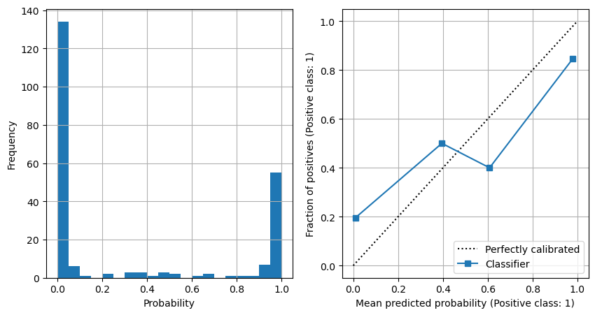
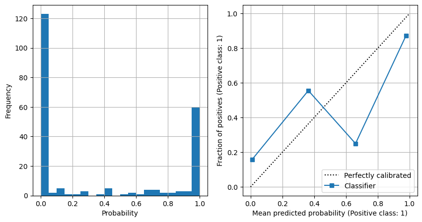
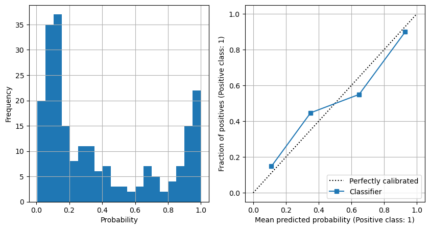
We would hope these three methods will give comparable results. While the final classification will be very similar, in this notebook we show that the reported probabilities are different, and that the single sigmoid output provides a much better calibrated model.
Load modules#
import matplotlib.pyplot as plt
import numpy as np
import pandas as pd

# sklearn for processing
from sklearn.preprocessing import MinMaxScaler
from sklearn.model_selection import train_test_split
from sklearn.utils import shuffle
from sklearn.calibration import CalibrationDisplay

# pytorch
import torch
from torch.autograd import Variable
import torch.nn.functional as F
Download data if not previously downloaded#
download_required = True

if download_required:

    # Download processed data:
    address = 'https://raw.githubusercontent.com/MichaelAllen1966/' + \
                '1804_python_healthcare/master/titanic/data/processed_data.csv'

    data = pd.read_csv(address)
    # Make all data 'float' type
    data = data.astype(float)

    # Create a data subfolder if one does not already exist
    import os
    data_directory ='./data/'
    if not os.path.exists(data_directory):
        os.makedirs(data_directory)

    # Save data
    data.to_csv(data_directory + 'processed_data.csv', index=False)
Define function to scale data#
In neural networks it is common to to scale input data 0-1 rather than use standardisation (subtracting mean and dividing by standard deviation) of each feature).
def scale_data(X_train, X_test):
    """Scale data 0-1 based on min and max in training set"""

    # Initialise a new scaling object for normalising input data
    sc = MinMaxScaler()

    # Set up the scaler just on the training set
    sc.fit(X_train)

    # Apply the scaler to the training and test sets
    train_sc = sc.transform(X_train)
    test_sc = sc.transform(X_test)

    return train_sc, test_sc
Load data#
data = pd.read_csv('data/processed_data.csv')
data.drop('PassengerId', inplace=True, axis=1)
X = data.drop('Survived',axis=1) # X = all 'data' except the 'survived' column
y = data['Survived'] # y = 'survived' column from 'data'

# Split into training and test
X_train, X_test, y_train, y_test = train_test_split(X, y, test_size = 0.25)

# Convert to NumPy arrays
X_train = X_train.values
X_test = X_test.values
y_train = y_train.values
y_test = y_test.values

# Scale data
X_train_sc, X_test_sc = scale_data(X_train, X_test)
1) SoftMax output with dual output#
Define neural net with Dual SoftMax output#
Dual output for died / survived, with SoftMax output.
class Net(torch.nn.Module):

    def __init__(self, number_features, expansion=2):
        # Define layers
        super(Net, self).__init__()
        self.fc1 = torch.nn.Linear(number_features, number_features * expansion)
        self.bn1 = torch.nn.BatchNorm1d(number_features * expansion)
        self.fc2 = torch.nn.Linear(number_features * expansion, number_features * expansion)
        self.bn2 = torch.nn.BatchNorm1d(number_features * expansion)
        self.fc3 = torch.nn.Linear(number_features * expansion, 2)

    def forward(self, x):
        # Define sequence of layers
        x = self.fc1(x) # Fully connected layer
        x = self.bn1(x) # Batch normalisation
        x = F.dropout(x, p=0.5) # Apply dropout
        x = F.relu(x) # ReLU activation
        x = self.fc2(x) # Fully connected layer
        x = self.bn2(x) # Batch normalisation
        x = F.dropout(x, p=0.5) # Apply dropout
        x = F.relu(x) # ReLU activation
        x = self.fc3(x) # Fully connected layer
        x = F.softmax(x, dim=1) # Softmax output (0-1, totals 1)

        return x
Train network#
# Define network
number_features = X_train_sc.shape[1]
net = Net(number_features)

# Set batch size (cases per batch - commonly 8-64)
batch_size = 16
# Epochs (number of times to pass over data)
num_epochs = 150
# Learning rate (how much each bacth updates the model)
learning_rate = 0.001
# Calculate number of batches
batch_no = len(X_train_sc) // batch_size

# Set up optimizer for classification
criterion = torch.nn.CrossEntropyLoss()
optimizer = torch.optim.Adam(net.parameters(), lr=learning_rate)

# Train model by passing through the data the required number of epochs

training_progress = []
test_progress = []

for epoch in range(num_epochs):

    # Shuffle the training data
    X_train_sc, y_train = shuffle(X_train_sc, y_train)

    # Set net to training mode
    net.train()

    for i in range(batch_no):

        # Get X and y batch data
        start = i * batch_size
        end = start + batch_size
        x_var = Variable(torch.FloatTensor(X_train_sc[start:end]))
        y_var = Variable(torch.LongTensor(y_train[start:end]))

        # These steps train the model: Forward + Backward + Optimize
        optimizer.zero_grad() # reset optimizer
        ypred_var = net(x_var) # predict y
        loss = criterion(ypred_var, y_var) # Calculate loss
        loss.backward() # Back propagate loss through network
        optimizer.step() # Update network to reduce loss

    # Set net to evaluation mode
    net.eval()

    test_var = Variable(torch.FloatTensor(X_train_sc))
    result = net(test_var)
    values, labels = torch.max(result, 1)
    y_pred_train = labels.data.numpy()
    accuracy_train = np.mean(y_pred_train == y_train)
    training_progress.append(accuracy_train)

    test_var = Variable(torch.FloatTensor(X_test_sc))
    result = net(test_var)
    values, labels = torch.max(result, 1)
    y_pred_test = labels.data.numpy()
    accuracy_test = np.mean(y_pred_test == y_test)
    test_progress.append(accuracy_test)
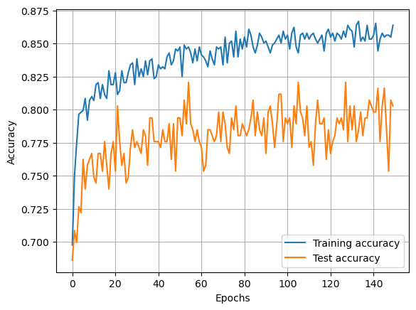
Show training
fig = plt.figure()
ax = fig.add_subplot()
x = np.arange(num_epochs)
ax.plot(x, training_progress, label='Training accuracy')
ax.plot(x, test_progress, label='Test accuracy')
ax.grid()
ax.legend()
ax.set_xlabel('Epochs')
ax.set_ylabel('Accuracy')
plt.show()
Show frequency of probabilities, and show model calibration#
net.eval()
test_var = Variable(torch.FloatTensor(X_test_sc))
result = net(test_var)
softmax_probs = result[:,1].data.numpy()

fig = plt.figure(figsize=(10,5))

ax1 = fig.add_subplot(121)
x = np.arange(num_epochs)
ax1.hist(softmax_probs, bins=20)
ax1.grid()
ax1.set_xlabel('Probability')
ax1.set_ylabel('Frequency')

ax2 = fig.add_subplot(122)
disp1 = CalibrationDisplay.from_predictions(
    y_test, softmax_probs, ax=ax2, n_bins=4)
ax2.grid()

plt.show()
2) Sigmoid output with dual output#
Define neural net with Dual Sigmoid output#
Dual output for died / survived, with SoftMax output.
class Net(torch.nn.Module):

    def __init__(self, number_features, expansion=2):
        # Define layers
        super(Net, self).__init__()
        self.fc1 = torch.nn.Linear(number_features, number_features * expansion)
        self.bn1 = torch.nn.BatchNorm1d(number_features * expansion)
        self.fc2 = torch.nn.Linear(number_features * expansion, number_features * expansion)
        self.bn2 = torch.nn.BatchNorm1d(number_features * expansion)
        self.fc3 = torch.nn.Linear(number_features * expansion, 2)

    def forward(self, x):
        # Define sequence of layers
        x = self.fc1(x) # Fully connected layer
        x = self.bn1(x) # Batch normalisation
        x = F.dropout(x, p=0.5) # Apply dropout
        x = F.relu(x) # ReLU activation
        x = self.fc2(x) # Fully connected layer
        x = self.bn2(x) # Batch normalisation
        x = F.dropout(x, p=0.5) # Apply dropout
        x = F.relu(x) # ReLU activation
        x = self.fc3(x) # Fully connected layer
        x = torch.sigmoid(x) # Sigmoid output (0-1)

        return x
Train network#
# Define network
number_features = X_train_sc.shape[1]
net = Net(number_features)

# Set batch size (cases per batch - commonly 8-64)
batch_size = 16
# Epochs (number of times to pass over data)
num_epochs = 150
# Learning rate (how much each bacth updates the model)
learning_rate = 0.001
# Calculate number of batches
batch_no = len(X_train_sc) // batch_size

# Set up optimizer for classification
criterion = torch.nn.CrossEntropyLoss()
optimizer = torch.optim.Adam(net.parameters(), lr=learning_rate)

# Train model by passing through the data the required number of epochs

training_progress = []
test_progress = []

for epoch in range(num_epochs):

    # Shuffle the training data
    X_train_sc, y_train = shuffle(X_train_sc, y_train)

    # Set net to training mode
    net.train()

    for i in range(batch_no):

        # Get X and y batch data
        start = i * batch_size
        end = start + batch_size
        x_var = Variable(torch.FloatTensor(X_train_sc[start:end]))
        y_var = Variable(torch.LongTensor(y_train[start:end]))

        # These steps train the model: Forward + Backward + Optimize
        optimizer.zero_grad() # reset optimizer
        ypred_var = net(x_var) # predict y
        loss = criterion(ypred_var, y_var) # Calculate loss
        loss.backward() # Back propagate loss through network
        optimizer.step() # Update network to reduce loss

    # Set net to evaluation mode
    net.eval()

    test_var = Variable(torch.FloatTensor(X_train_sc))
    result = net(test_var)
    values, labels = torch.max(result, 1)
    y_pred_train = labels.data.numpy()
    accuracy_train = np.mean(y_pred_train == y_train)
    training_progress.append(accuracy_train)

    test_var = Variable(torch.FloatTensor(X_test_sc))
    result = net(test_var)
    values, labels = torch.max(result, 1)
    y_pred_test = labels.data.numpy()
    accuracy_test = np.mean(y_pred_test == y_test)
    test_progress.append(accuracy_test)
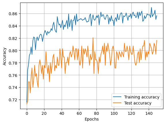
Show training
fig = plt.figure()
ax = fig.add_subplot()
x = np.arange(num_epochs)
ax.plot(x, training_progress, label='Training accuracy')
ax.plot(x, test_progress, label='Test accuracy')
ax.grid()
ax.legend()
ax.set_xlabel('Epochs')
ax.set_ylabel('Accuracy')
plt.show()
Show frequency of probabilities, and show model calibration#
net.eval()
test_var = Variable(torch.FloatTensor(X_test_sc))
result = net(test_var)
softmax_probs = result[:,1].data.numpy()

fig = plt.figure(figsize=(10,5))

ax1 = fig.add_subplot(121)
x = np.arange(num_epochs)
ax1.hist(softmax_probs, bins=20)
ax1.grid()
ax1.set_xlabel('Probability')
ax1.set_ylabel('Frequency')

ax2 = fig.add_subplot(122)
disp1 = CalibrationDisplay.from_predictions(
    y_test, softmax_probs, ax=ax2, n_bins=4)
ax2.grid()

plt.show()
3) Single sigmoid output#
Define neural net with single Sigmoid output#
One outut for probability of survival
class Net(torch.nn.Module):

    def __init__(self, number_features, expansion=2):
        # Define layers
        super(Net, self).__init__()
        self.fc1 = torch.nn.Linear(number_features, number_features * expansion)
        self.bn1 = torch.nn.BatchNorm1d(number_features * expansion)
        self.fc2 = torch.nn.Linear(number_features * expansion, number_features * expansion)
        self.bn2 = torch.nn.BatchNorm1d(number_features * expansion)
        self.fc3 = torch.nn.Linear(number_features * expansion, 1)

    def forward(self, x):
        # Define sequence of layers
        x = self.fc1(x) # Fully connected layer
        x = self.bn1(x) # Batch normalisation
        x = F.dropout(x, p=0.5) # Apply dropout
        x = F.relu(x) # ReLU activation
        x = self.fc2(x) # Fully connected layer
        x = self.bn2(x) # Batch normalisation
        x = F.dropout(x, p=0.5) # Apply dropout
        x = F.relu(x) # ReLU activation
        x = self.fc3(x) # Fully connected layer
        x = torch.sigmoid(x) # Sigmoid output (0-1)

        return x
Train network#
# Define network
number_features = X_train_sc.shape[1]
net = Net(number_features)

# Set batch size (cases per batch - commonly 8-64)
batch_size = 16
# Epochs (number of times to pass over data)
num_epochs = 150
# Learning rate (how much each bacth updates the model)
learning_rate = 0.001
# Calculate number of batches
batch_no = len(X_train_sc) // batch_size

# Set up optimizer for classification
criterion = torch.nn.BCELoss()
optimizer = torch.optim.Adam(net.parameters(), lr=learning_rate)

# Train model by passing through the data the required number of epochs

training_progress = []
test_progress = []

for epoch in range(num_epochs):

    # Shuffle training data
    X_train_sc, y_train = shuffle(X_train_sc, y_train)

    # Set net to training mode
    net.train()

    for i in range(batch_no):

        # Get X and y batch data
        start = i * batch_size
        end = start + batch_size
        x_var = Variable(torch.FloatTensor(X_train_sc[start:end]))
        y_var = Variable(torch.FloatTensor(y_train[start:end]))

        # These steps train the model: Forward + Backward + Optimize
        optimizer.zero_grad() # reset optimizer
        ypred_var = net(x_var) # predict y
        loss = criterion(ypred_var, y_var.reshape(-1,1)) # Calculate loss
        loss.backward() # Back propagate loss through network
        optimizer.step() # Update network to reduce loss

    # Set net to evaluation mode
    net.eval()

    test_var = Variable(torch.FloatTensor(X_train_sc))
    result = net(test_var)
    values = result.data.numpy().flatten()
    y_pred_train = values >= 0.5
    accuracy_train = np.mean(y_pred_train == y_train)
    training_progress.append(accuracy_train)

    test_var = Variable(torch.FloatTensor(X_test_sc))
    result = net(test_var)
    values = result.data.numpy().flatten()
    y_pred_test = values >= 0.5
    accuracy_test = np.mean(y_pred_test == y_test)
    test_progress.append(accuracy_test)
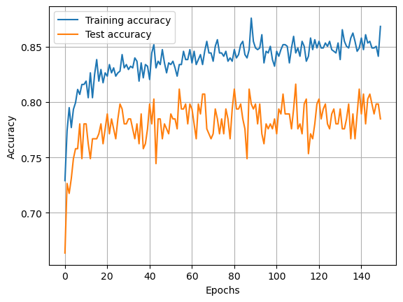
Show training
fig = plt.figure()
ax = fig.add_subplot()
x = np.arange(num_epochs)
ax.plot(x, training_progress, label='Training accuracy')
ax.plot(x, test_progress, label='Test accuracy')
ax.grid()
ax.legend()
ax.set_xlabel('Epochs')
ax.set_ylabel('Accuracy')
plt.show()
Show frequency of probabilities, and show model calibration#
net.eval()
test_var = Variable(torch.FloatTensor(X_test_sc))
result = net(test_var)
sigmoid_probs = result.data.numpy().flatten()

fig = plt.figure(figsize=(10,5))

ax1 = fig.add_subplot(121)
x = np.arange(num_epochs)
ax1.hist(sigmoid_probs, bins=20)
ax1.grid()
ax1.set_xlabel('Probability')
ax1.set_ylabel('Frequency')

ax2 = fig.add_subplot(122)
disp1 = CalibrationDisplay.from_predictions(
    y_test, sigmoid_probs, ax=ax2, n_bins=4)
ax2.grid()

plt.show()
Observations#
A single sigmoid output produces the best calibrated model